Field Activity #2: Visualizing and Refining Your Terrain Survey

INTRODUCTION

This is the second part of a two week exercise in which groups of students were to make landscapes in the snow, collect elevation data, and make 3D models of the terrain. First, the landscape needed to be made and coordinate system set up. With that accomplished, elevation data could be collected using meter sticks, string, and a little ingenuity. At this point, part 1 of the exercise was completed. A more in-depth view of these procedures can be seen in my last blog post, Field Activity #1: Creation of a Digital Elevation Surface Using Critical Thinking Skills and Improvised Survey Techniques.

In this part of the exercise, the elevation data taken in part one will be entered into excel, imported into ArcMap or ArcScene, and used to create 3D models by utilizing different interpolation methods. Five different surfaces will be compared and the best method will be chosen.

METHODS

Now that the elevation data was collected, it could be entered into an excel spreadsheet with column headers of “x”, “y”, and “z”. The lowest number collected was -12 and as such 12 was added to each elevation sample to eliminate any negative numbers and make the data set easier to work with.

Figure 1: The excel file that holes all the x,y,z data for the landscape. After importing the sheet into ArcScene the data was displayed as XY data and converted into a shape file to be used for interpolation methods.

With the excel sheet in the proper format, it could then be imported into either ArcMap or ArcScene to experiment with different interpolation methods. The excel file was imported into ArcScene and converted into a shape file by first displaying the XY data and then exporting the data as a point shape file.

Figure 2: This is what the XY data and the resulting shape file looked like from an overhead veiw in ArcMap or Arc Scene. In ArcScene the Z data also comes into play and the points are shown at their relative heights.

With the data in the proper format in ArcScene, different interpolation methods could be used to visually and spatial analyze the landscapes elevation.  Five different methods were used: IDW, Kriging, Natural neighbor, Spine, and TIN. These can be preformed by navigating to the ArcToolbox > 3D Analyst Tools > Raster Interpolation. To make a TIN navigate to the ArcToolbox > 3D Analyst Tools > Data Management > TIN. An interpolation method uses sample data points, in this case elevation points of the landscape, and creates a raster in which it predicts what values the adjacent cells would have based on different parameters. There are two types of interpolation methods, deterministic and geostatistical. Deterministic methods base their predictions on measured values and mathematical formulas, while geostatistical methods use statistical models to predict surfaces.

IDW (Inverse Distance Weighted)

This interpolation method estimates values by averaging the data in groups centered on a processing cell. As such, it is a deterministic method. A group of points and their accompanying processing cell is called a neighborhood. More weight is given to points closer to the center of the processing cell. Points farther away from the processing cell are assumed to have less influence. The manner in which IDW interpolates can be altered by changing the number of processing cells or by specifying the radius the neighborhood will take.

Figure 3: The surface interpolated using the IDW method. This method fit the survey the poorest. The surface has many peaks and depressions that are not present in the actual landscape.

Kriging

The kringing method is somewhat complex and uses statistics to predict surfaces, making it a geostatistical method, with a level of accuracy and certainty that is not possible with deterministic interpolation methods. This method assumes there is a spatial correlation between points based on their distance and direction to each other to create a surface. This method is best used when a distance or directional bias is known or assumed about the data. This method is best used for soil science and geology.

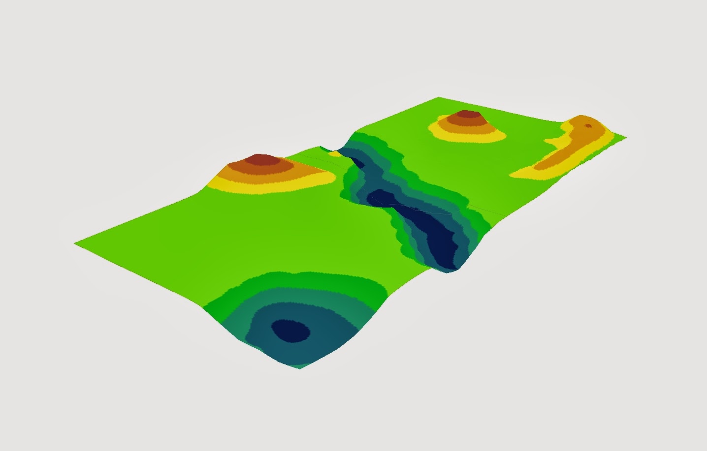
Figure 4: The surface interpolated using the Kriging method. This method fit the surface well. The mountain peaks are curved and the river bed is continuous and drops in elevation properly.

Natural Neighbors

This interpolation method uses area to apply varying weights to sample data that surround a query point. The surface created will pass through all sample points and will not produce any peak, pit, ridge, or valley that is not explicitly present in the data used. Unlike IDW, the weights given are based on overlapping area and not distance. However, like IDW, Natural Neighbors is a deterministic method.

Figure 5: The surface interpolated using the Natural Neighbors method. This method fit the survey well but not as well as others. The mountain peaks are a bit to pointed and the ridge is lacking in elevation.

Spline

Being another deterministic method, the Spline method uses a mathematical function to create a surface that passes through each point minimizing surface curvature for the entire area. The surface created will be smooth and will pass through each sample point exactly. There are two types of Spline interpolation, regularized and tension. Regularized creates a smooth surface with values that could extent past the data range, while tension creates a less smooth surface but will have values that fall within the data range. This method is best used for elevation, water table heights, and pollution concentrations.

Figure 6 (1): The surface interpolated using the Spline method. This method fit the survey the best. By running the surface through each point taken, the resulting model represents what the snow landscape actually looked like.

TIN (Triangulated Irregular Network)

A TIN surface is constructed by placing vertices at the sample points and connecting these vertices with edges to form triangles. The resulting network of contiguous triangles models the values between points without changing the position of the sample data. This method is best used for areas with a high degree of irregularity.

Figure 7: The surface interpolated using the TIN method. This method fit the survey but is less visually pleasing then other methods. The snow landscape did not have straight edges however the look of the surface is simply a side effect of the method used. By creating a network of triangles, the majority of curvature in the landscape was lost.

DISCUSSION

Of all five interpolation methods, IDW (Figure 3) fit the survey the poorest. Each point dips down or protrudes up in a fashion that does not correlate with what the landscape actually looked like. The mountain peaks consist of multiple peaks instead of just one and the river valley is littered with recesses that make the surface resemble Swiss cheese. The Nearest Neighbor (Figure 5) method fit the survey better but consists of too many rigid and sharp edges. The mountain peaks, ridge top, and river valley were not as pointed as this method would suggest.

The TIN (Figure 7) method for the landscape does fit the survey but in a more abstract fashion. The rigidness of the features is somewhat visually displeasing but is simply a side effect of the method. The mountains and ridges fit better than the river valley and lake depression. The area around the river valley is very blocky with straight lines that do not correlate with the actual landscape. More samples of elevation points are needed to make this method more viable.

The Kriging (Figure 4) method fit the survey very well with the only exception being the ridge top. The surface has multiple tips on the ridge when in reality the ridge has a smooth top. The river valley has a smoother and more continuous bottom and the mountain peaks are more curved when compared to the IDW (Figure 3), TIN (Figure 7), and Nearest Neighbor (Figure 5) methods, which correlate better to the actual landscape.

The Spline (Figure 6) method fit the survey best. The mountain peaks are curved yet still reach the proper height and retain their proper shape. The ridge top is curved and continuous. All the features are portrayed with the proper amount of curve and look the way the landscape should. This method also captured the slight ridge around the river valley better than the other methods did. The only problems are slight depressions around the ridge and in the river valley. This may be caused by improper sampling technique or it may be realistic to the actual surface. The area appears flat in person, however the data suggests otherwise and it can be difficult to tell minute changes in elevation when starring at all white snow.

Figure 6 (2): The surface interpolated using the Spline method. This surface represented the actual landscape the best of all five methods used. The mountains and ridge are peaked yet curved, the river valley curves and drops in elevation like it should, and overall the model fits the survey well.

CONCLUSION

After experimenting with different interpolation methods and analyzing the surfaces created, it was decided that the Spline (Figure 6) method represented the landscape best. This would make sense given the fact that the spline method creates a surface that passes through each sample point and gives the surface a smooth appearance. Using snow as the construction medium resulted in smooth curved features which was represented best with the Spline (Figure 6) method, decently with the Nearest Neighbor (Figure 5) and Kriging (Figure 4) methods, and poorly with the IDW (Figure 3) and TIN (Figure 7) methods. Taking more sample points would result in better surfaces for all methods, although each method except for IDW (Figure 3) produced surfaces that did represent the landscape well. Due to time and schedule restraints a re-survey was not possible. Had a re-survey been done the results would be incomparable due to changes in the landscape from more snow falling and wind caused snow drifts.

Using the top of the box as sea level and using a slightly distorted coordinate system was not in itself a major contributor to error in the surfaces created. More sample points in areas with swift changes in elevation were needed to create better representations of the landscape. Though the measurement method was slightly flawed, the models made in ArcScene do correlate with the landscape and look pretty neat.

Group #2 did an excellent job of working together to get part one of the exercise complete. However, it was harder to come together for part two. We were unable to arrange a re-survey which would have improved our results and a lack of communication was to blame. I learned quite a bit about the different interpolation methods offered in ArcMap and ArcScene from this exercise, as well as how to take data from the field and create useful models. The group’s inability to come together at the end of the exercise is a good reminder to start working early and communicate often. Despite the horridly frigid weather, this exercise was enjoyable, thought provoking, and open ended enough to feel like the students were not being simply walked through another assignment.