Equipment Day

This week for class, students went outside for an equipment day to become familiar with different mediums for capturing aerial imagery. After researching UAV technology earlier in the semester, it was time to get some hands on experience with two different rotary crafts, along with a 9-foot kite and a small rocket.

 

Figure 1:  This rotary craft was funded by our professor, Joe Hupy, and built by a physics student, Max, still attending UWEC. Rotary wing crafts are known to have short flight times and as such this craft was built with payload in mind. This craft has a flight time of about 15 minutes at best but can also carry more equipment and sensors than others its size.

 

Figure 2: This is Max preforming the calibration flight for Joe's UAV. The craft jerked around back and forth testing and calibrating the different motors and electrical pieces. It stayed in the air for about 8 minutes and then made a safe landing back on the sidewalk.

 

 Figure 3: This is the heads-up-display (HUD) for Joe's UAV. There is a small sensor on the front of the craft that transmits a first person view of what the craft sees back to the headset. The headset also displays assorted flight information.

 Figure 4: This is Max's own rotary craft, built by himself and funded by the University. Max was more comfortable with his own craft and showed off his skills in UAV piloting by spinning the craft around in the air and racing it at top speed nearly touching the ground.

 Figure 5: A comparison shot of both rotary crafts. The camera seen mounted on the front bottom of Joe's craft is for taking the aerial imagery. A regular camera was used for low cost and ease of use. Smaller sensors that comprise nothing but the actual sensor itself, not actual cameras, are ideal for optimizing the payload capacity of a UAV.

 Figure 6: Here is Joe's 9-foot kite. Setup is very easy consisting of proper placement of 2 metal bars. On moderatly windy days, a camera can be attached to the string to capture aerial imagery. On days that have very little to no wind, a balloon can be used instead.

 Figure 7: Here the camera can be seen. It was just attached and will be let up at least another 100 feet before imagery will be collected. Wind is needed to get the kite into the air and keep it there, however, too much wind will blow the camera around and the quality of imagery may be compromised.

 Figure 8: The final experiment of the day was a mini rocket. Only half the fuel for the rocket ignited which resulted in somewhat of an anticlimactic ending to the day. Small sensors were taped on the sides of the rocket to take pictures every second or so. The rocket did not achieve a proper height to collect any meaningful imagery.

Activity #6: Microclimate Geodatabase Construction for Deployment to ArcPad

Introduction

This activity will be broken down into two parts. The first will be an explanation of the importance of proper mission planning in regards to data collection and the second will be a walkthrough of how to set up a geodatabase with proper domains. Later the geodatabase that is created will be used to collect data on Microclimates here on the UWEC campus.

Part I - Proper Mission Planning for Data Collection

Before heading out to the field to collect data, it is crucial to fully understand what features are going to be collected and what attributes about them should be stored. Data can be represented different ways in a computer and each data type has its purposes and limitations. Understanding this concept can help determine the best data type for whatever features are being collected. Regardless of the specifics, it is always a good idea to store the data in a file geodatabase. A file geodatabase is essentially a system folder that reads and manages geospatial data. There are multiple advantages to using a file geodatabase, which is best described by ESRI here.

There are six data types or field types available when creating a file geodatabase; short integer, long integer, float, double, text, and date. Taken from ArcGIS Desktop Help:

Data type	Storable range	Size (Bytes)	Applications
Short integer	-32,768 to 32,767	2	Numeric values without fractional values within specific range; coded values
Long integer	-2,147,483,648 to 2,147,483,647	4	Numeric values without fractional values within specific range
Float (single-precision floating-point number)	approximately -3.4E38 to 1.2E38	4	Numeric values with fractional values within specific range
Double (double-precision floating-point number)	approximately -2.2E308 to 1.8E308	8	Numeric values with fractional values within specific range

ArcGIS data types table

Data type: Text – the field will represent a series of alphabetic symbols. The Text type is what you would expect, it enables the storage of words through the use of written language.

Data type: Date – used to store dates and/or times. The default format is mm/dd/yyy hh:mm:ss and a specification of AM or PM.

When deciding what numeric data type to use, it is best to choose the type that will minimize storage space. If the values collected are expected to range from 1 to 1,000, the short integer data type would be most appropriate. If the values collected are expected to reach numbers that exceed 4 billion that Float would be most appropriate. Another consideration to make is the precision of the data collected. Float will only store 6 decimal positions while double will store 15.

After the data type is chosen the domain type can be selected. There are two chocies for domain type: Range and Coded Values. Each data type can be associated with either domain type except for text, which requires Coded Values. Range lets the user define a range of numbers that the data must fall within. This can help reduce user input error. When creating a domain for temperature data, the user may want to make the range 0-99 (for Fahrenheit) if they are confident that the temperature will not be less than 0 or more than 99. That way when the user is collecting data and accidentally adds an extra digit, entering 455 instead of 45, the data will automatically be rejected minimizing confusion and effort later on when analyzing the data. The next option is Coded Values. For this type, a numeric or textual “code” can be attached to a more robust description. This is useful for recording a simple cardinal direction of North, East, South, or West for example. Instead of entering the full direction name for each sample, coded values would allow just an “N” for North or “S” for South, minimizing collection time and tediousness.

After the desired domains are created, a feature class(es) can be made with descriptive fields. The fields created will need to have a data type selected just like the domains. This data type selection is important because it will determine the domains that are available. Each field will be given a domain and multiple fields can have the same domain. The fields are what will be used when the data is collected and the domain attached to the field will determine the criteria the data will need to fulfill.

Part II - Geodatabase Creation

ArcCatalog will be used to create and modify the geodatabase. To create a geodatabase right-click the destination folder, hover the mouse over New, and choose File Geodatabase.

 

 

Figure 1: After creating a file geodatabase this is what the screen will look like.

Figure 2: Right click on the file geodatabase and choose properties. The Database Properties window will appear. The data type or field type can be chosen via the highlighted dropdown menu. Notice the six data types discussed earlier.

 

 

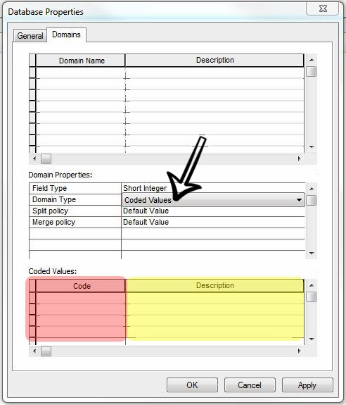
Figure 3: With the domain type as Coded Values, the red highlighted portion of the window is where the "code" is entered (N for North, 1 for Group 1, etc.) and the yellow highlighted portion is where a description of the code goes (North describes N, Group 1 describes 1, etc).

Figure 4: With the domain type as range, the maximum and minimum values can be entered in the red highlighted portion of the window.

 

 

 

 

Figure 5: Once the geodatabase and desired domains are created, a new feature class can be made. The type of features can be chosen from the drop down menu. Click next after naming the feature class and selected its type.

 

 

Figure 6: Next the coordinate system can be established or changed. Once the proper coordinate system is chosen click next. Click next on the next two windows that appear and the fields for the feature class can be created.

 

 

Figure 7: Type the name of the desired field in the Field Name section of the table. These names are what will be used in the field for data collection, so make these names recognizable and distinguishable. The arrow pointing at "Float" in the data type and the arrow pointing at Temp in the Domain dropdown box, show the relation between filed data type and available domains. The only domain with the Float data type is Temp and is therefore selectable with fields that also have the Float data type.

 

 

Figure 8: These are the final domains that were created for the future UWEC Microclimate survey. Group has a short integer data type with coded values (notice the values at the bottom of the window). Relative_Hum has a float data type with a range of 0 to 100 (because it is a percent). Snow_Dep has a float data type with a range of 0 to 36 (assumed max height of snow is a meter stick in inches). Temp has a float data type with a range of -20 to 99 (assuming temperature will not go below -20 degrees anymore and not over 99). Time has a short integer data type with a range of 0 to 2400 (for recording military time). Wind_Dir has a text data type with coded values (N = North, NE = Northeast, etc). Wind_Spd has a short integer data type with a range of 0 to 60 (assuming wind speeds will not exceed 60 mph)

 

 

 

 

Figure 9: These are the final fields created for the future UWEC Microclimate survey. Many of the fields have similar names to the domain they will be defined by. Besides those, Dew_Point will use the Temp domain and Notes has no domain. Notes will be used for entering any useful information in the field that may be good to know later on (such as noticeable anomalies, mistakes, etc.). 

 

Activity #5: Learning Distance Bearing Navigation and Development of a Field Navigation Map

Introduction

In this exercise, students will learn the basics of field navigation using only a map and compass. After having learned how to properly use a compass, two maps will be made with grids displaying different coordinate systems. One map will have a geographic coordinate system (lat/long) and the other will have a projected coordinate system in UTM. The maps will contain the same area, The Priory in Eau Claire, WI, and will be used for actual field navigation later in the semester. The two types of coordinate systems will then be compared and analyzed.

Methods/Discussion

- Learning Distance Bearing Navigation-

A compass is one of the most basic navigation instruments available and works with any map or as a stand-alone device. The simplest explanation for what a compass is would be a strip of metal that is floating in liquid that reacts to the earths magnetic field so that the red portion of the metal strip points towards magnetic north. There are different kinds of compasses but the focus of this exercise is on the orienteering compass.

Figure 1: An orienteering compass. Each part is labeled. The base plate and compass dial are clear. The magnetic needle will be red and white. The orienting arrow and direction of travel arrow may be red or black depending on the style of compass.

There are essentially three main components of a basic orienteering compass: the clear baseplate, rotating compass dial, and a magnetic needle. On the baseplate there is a direction of travel arrow and an index line. Inside the rotating compass there is an orienting arrow and meridian lines. Surrounding the rotating compass are degree ticks and the four cardinal directions. The magnetic needle has two sides, the red side is north and the white is south. All the functions of each part of the orienteering compass will be described later.

To begin, the compass shows the four cardinal directions: North, East, South, and West. Each cardinal direction corresponds with a specific degree, see figure 2. Understanding these numbers can quickly help determine if the correct bearing is taken when in the field.

Figure 2: The cardinal directions are colored red. The compass can be broken down into smaller increments (NNE, NE, ENE, etc.) then the 90 degree brakes of the cardinal directions and are labeled on the figure.

A bearing is the direction, measured in degrees from magnetic north, form one location to another. To take a bearing, hold the compass straight out in front, with the direction of travel arrow pointed towards the location of interest, and hold it steady. Then rotate the compass dial until the red (north) portion of the magnetic needle is within the orienteering arrow (see figure 1). The number that is now posited at the Index line is the bearing. Following this bearing will lead to the location of interest. This technique is used in the field when the location can be viewed with a persons eye.

Figure 3:Finding a
bearing from a map. 

When the location is too far away or too hidden by obstacles to be seen, or simply a position drawn on a map, the orienteering compass can be used along with a map to find the bearing. Assuming there are two places are known on the map, a start and end, the bearing can be found. Place the compass on the map with the direction of travel arrow pointing from the starting position to the ending position. Try and get the direction of the compass to fall as accurately as possible through the two points, use a straight edge and pencil if needed. Then turn the compass dial so that the orienteering arrow is pointed straight up, or to the north. If the map has a grid, the meridian lines in the compass dial can be lined up to increase the accuracy. With the orienteering arrow pointing north and the compass still pointing towards the ending point, the bearing can be recorded (the number at the Index line).

Just like when taking azimuth data in the previous exercise, magnetic declination comes into play, when using a compass and map. When using a map drawn to true north to find declinations to use in the field, it is important to either add or subtract the declination of the area of interest from the map bearing. The magnetic declination for Eau Claire,WI was calculated earlier in Field Activity #4: Conducting a Distance Azimuth Survey., and is 1.08139 W and as such should be added to each map bearing.

Knowing how to use a map and compass is not the only skill needed to successfully naviate in the field. Establishing a pace count is also important. A pace count is the number of paces it takes to cover a known distance, typically 100 meters. A pace is the distance covered each time one foot (the individual decides either the right or left) hits the ground. My pace count for 100 meters is 63. Having established a pace count, a person can roughly estimate the distance traveled along their bearing.

A handy technique to make things easier when navigating the field is to find a feature (tree, statue, anything recognizable, etc.) that falls along the map bearing and travel towards that instead of constantly watching the compass. At times there may be impassable features (pond, marsh, endangered animal habitat, etc.) along the bearing and there are several methods to bypass this issue. The first is finding a feature along the bearing like stated above, and walk around the impassable feature to the known feature along the bearing and continue. If there is no feature along the bearing, and multiple people are in the field then a person can walk around the impassable feature and become the known feature along the bearing (making sure to take a back bearing to be sure the individual is along the bearing line). If there is only one person in the field, then that individual can approach the impassable feature and turning 90 degrees multiple times, walk around the impassable feature taking a pace count for each direction traveled. By walking the same distance back  to the bearing line as the person walked away from the bearing line will result in the individual being at least roughly back on track. See figure 4 for an illustration of this technique.

Figure 4: How to deal with an impassable feature when following a map bearing. Keeping track of a persons pace and turning 90 degrees three times will result in knowing roughly the distance traveled pass the feature and will result in the person being back along their map bearing.

Any questions regarding using a map and compass that are not addressed here are most likely found at this website: Compass Basics: An Introduction to Orientation and Navigation  All pictures were taken from this website.

- Development of a Navigation Map - 

 

 The next task for this exercise is to create two maps of the Priory in Eau Claire, WI, to be used later in the semester for actual field navigation. These maps were created in ArcMap 10.2 and used data from the UWEC Geography department. Each map needed certain criteria (grid, proper size, north arrow, data sources, etc.) but it was up to the student to decide what to include on the map itself. When creating a map for field navigation, it is vital to include only what is needed as superfluous data can cause the map to become cluttered and difficult to read. Because of this, I choose to include 5 meter contours and a semi-transparent DEM (digital elevation model). Using these two layers, the topography of the Priory is easily distinguishable without making the map too busy, which the addition of aerial imagery often does.

 

Figure 5: The DEM of Eau Claire, WI used for the maps, and for creation of the 5 meter contour lines. The small orange/brown box that can be seen in the upper portion of the DEM is the Priory study area.

 

 

It began with a raster based DEM, which means the model is made up of a grid of squares with each square having a height value and representing a different color. Using the Contour tool in the ArcToolbox  under Spatial Analyst Tools >  Surface > Contour, contour lines of varying size can be created. For this map, 5 meter spacing was chosen.

 

Figure 6: The Contour Tool and it's location. Here different rasters can be chosen and the size of the contours can be decided.





 

After the contours were made, they were clipped to appear only the study area using the Clip Tool found in the ArcToolbox under Analysis Tools > Extract > Clip. The layer to be clipped was the recently created 5 meter contour shape file and the layer to clip from was a navigation boundary polygon from the Geography Department.

 

Figure 7: The Clip Tool. Used to clip a feature within the boundaries of another. Used to clip 5 meter contour lines to within the study area, since the lines outside the study area were not relevant to the exercise.

 

 

 

Figure 8: The resulting clipped contour lines, semi-transparent DEM (by changing the display options by right clicking the layer and choosing Properties > Display), and the study area polygon.

 

 

 

Now the work in Data View was done and the Layout was assembled. Each map needed: a north arrow, a scale bar and absolute scale, geographic and projected coordinate systems, data sources, name, date, watermarks, and a grid displaying a geographic coordinate system  for one and a projected UTM coordinate system for the other. To add a grid, right click inside the data frame and choose Properties > Grids. At this point new grids can be created or existing grids can be turned on or off. Clicking "New Grid..." will the Grids and Graticules Wizard window in which three different types of grids can be created. The geographic coordinate system map was made with the Graticule option and the project coordinate system map was made with the Measured Grid option. Going through the wizard allows the user to change the appearance of the lines and division ticks. Once the grid is created the labels can be formatted accordingly.

 

Figure 9: Creating a new grid. The window on the left is the Data Frame Properties where the user can select pre-existing grids or make a new one. The window on the right is the Grids and Graticules Wizard window which will guide the user through making a new grid.

 

 

Figure 10: By highlighting a grid and clicking the Properties... option in the Data Frame Properties window, another window appears that lets the user customize the options for the grid. Most importantly for this exercise the labels can be changed in the Labels tab. All the options for labels are expanded and shown in this figure.

 

 

The rest of the criteria for the map was added by clicking the Insert tab on the main toolbar and choosing the appropriate item.

  

 

 Figure 11: The map with the grid displaying a geographic coordinate system.

Figure 12: The map with the grid displaying a project coordinate system.

 

 

The reason two maps were created is to compare the effectiveness of each type of coordinate system in preforming field navigation. Geographic coordinate systems are good for small scale maps and looking at features on a broad scale, while projected coordinate systems are best used for large scale maps and examining features at a finer scale. It would be assumed that the map with the UTM projected system would be better for the purpose of the field navigation activity later in the semester.





 

 

Field Activity #4: Conducting a Distance Azimuth Survey.

Introduction

These days there are many ways to survey an area, but sometimes the most convenient technological method will be either unavailable or unpractical. In these situations it is critical for a field technician to understand and utilize basic survey techniques that relay less on technology or expensive clunky equipment and more on geographic knowledge and ingenuity. For this exercise, students will work in groups of 3 to survey an area of their choosing with a TruPulse 360/B range finder. This piece of equipment will let students record slope distance and azimuth for a number of locations in their chosen area.

Figure 1: TruPulse 360/B. Measures distances, heights, and azimuth. Can integrate with GPS and has Bluetooth capabilities. LTI 360 degrees TruVector Compass Technology. lasertech.com

Along with recording slope distance and azimuth, students will also record an attribute of each point (height, diameter, type, etc.).By carefully choosing survey points and using either GPS technology or aerial image interpretation, students will be able to also include a starting survey point for each point collected. Once all the data is entered into an excel spreadsheet, it can be imported into ArcMap and models can then be made and discussed.


Methods/Discussion

Firstly, when working with azimuth in surveying it is important to know the magnetic declination from true north. Magnetic declination is the angle between magnetic north (magnetic pole) and true north (geographic pole). It is important to know that magnetic declination changes by location and also over time. By utilizing this website set up by NOAA, anyone can calculate their magnetic declination. In Eau Claire, WI the magnetic declination is 1 degree 4 minutes and 53 seconds W (-1.08139 W in decimal degrees).

Figure 2: The magnetic declination for Eau Claire, WI generated by NOAA at this website. The magnetic declination will be added to the azimuth measurements taken in the field to increase the accuracy of the final results.

In determining whether to add or subtract this declination from the azimuth data collected, the mannerism "East is least and West is best" can be used. When dealing with a declination to the east, the value should be subtracted from the azimuth. When the declination is to the west, the value should be added to the azimuth. Therefore, for Eau Claire, WI, the declination of 1.08139 should be added to each azimuth recorded.

The study area chosen was Wilson Park, both due to its size and proximity to campus/individuals housing. The park takes up one city block near downtown Eau Claire and has multiple trees, benches, tables, electrical boxes, signs, statues, and electrical posts. The attribute collected for each point reflects the type of object found at that location (tree, sign, etc.). The goal of this survey was to measure each feature inside the one block area of Wilson Park. Three different survey positions were used and the locations of each were chosen near a permanent structure that would be easy to find on an aerial image, for when coordinates were needed later.

Figure 3: Survey position A on the corner of Emery and Farwell. This spot was chosen due to the electrical pole that would be easy to find on aerial imagery allowing the coordinates to be determined without using GPS technology.

 

 

 

Figure 4: The view from survey position A. Trees blocked the line of sight to a good portion of the park so multiple survey positions became mandatory.

 

 

 

Figure 5: Survey position B on the corner of Earl and Farwell. This spot was chosen due to the fire hydrate that would be easy to spot on aerial imagery. This spot was originally going to be located near an electrical pole, like the first, however a bus spot was located at that position and buses keep stopping for us to get on.

 

 

Figure 6: The view from survey position B. The area hidden behind trees at survey position A is now visible and the features in this portion of Wilson Park can be measured.

 

 

Figure 7: The view from survey position C on the corner of Earl and Barstow. This spot was chosen due to an electrical pole that would be easy to find in aerial imagery. The last remaining features of Wilson Park could be measured from this position and as such, position C was the last survey position used.

 

 

 

With the data collected, it could then be entered in an Excel spreadsheet in the proper format. The resulting table had 6 fields: "pnt_numb" indicating the number of each point as it was taken, "pnt_type" indicating which kind of feature is found there, "sdist" indicating the slope distance, "azi" indicating the azimuth, and finally "X" and "Y" indicating the x,y coordinates in decimal degrees to 6 decimal places (suggested format). 

Figure 8: A sample from the excel spreadsheet. The degrees have 6 decimal places by suggestion of the professor. Last time the class was taught, students tried using less decimal places and ArcMap would error when the Bearing Distance To Line tool was used.

The above screen capture of the final spreadsheet had to be modified multiple times before it arrived at its current state and could be used in ArcMap. The original table I used did not have azimuth data corrected for magnetic declination, had slightly wrong survey positions (X,Y values), and also had one row at the bottom with null values. Simply adding 1.08139 to the azimuth values corrected the first problem. For the second problem, at first, the survey positions were found via Google Earth and converted into decimal degrees. When the data was imported into ArcMap the survey positions were just slightly off. So, ArcMap itself was used to collect the survey position values by adding an aerial imagery base map and going to [Customize - ArcMap Options... - Data View]. Here the units displayed on screen could be set to decimal degrees with 6 decimal places. The final problem was most frustrating to figure out. The null values in the table made ArcMap error when the Bearing Distance To Line tool was used. It took awhile to figure this out but once the data was entered into a new clean spreadsheet with no null values the Bearing Distance to Line tool worked perfectly.

 

A geodatabase was created in ArcMap to hold all the files pertaining to this lab. This was done by rightclicking the desired folder in the Catalog window, hovering over New..., and choosing File Geodatabase. Once the geodatabase was created, the excel table was imported into it by rightclicking the geodatabase, hovering over Import..., and selecting Table (single). Next the ArcToolbox contains the two tools needed to take the data collected from the field and display it on a computer: Bearing Distance To Line and Feature Vertices To Points.

 

 

Figure 9: The ArcToolbox with relevant tools highlighted in red.

 

 

 

Figure 10: The Bearing Distance To Line dialog box. Here the table imported into the geodatabase is selected, its output location is selected, and its different fields are placed in the appropriate sections.

 

 

 

Figure 11: This is the result after the Bearing Distance To Line tool ran successfully. A line shapefile was created that illustrates where each feature measured relates to its survey position.

 

 

 

Figure 12: Next the Feature Vertices To Points tool was run. The line shapefile create earlier is selected and all vertices receive a point, creating a point shapefile for each of the features measured.

 

 

 

Figure 13: This is the result after the Feature Vertices To Points tool ran successfully. Both new shapefiles are present and aerial imagery can now be placed underneath to give some context to what the feature are.

Figure 14: With aerial imagery of Wilson Park underneath the shapefiles, the effectiveness of the survey method can be analyzed.

Conclusions

 

Upon examination of the final product (Figure 14), it can be determined that several things went wrong during data collection. The goal of this survey was to measure each individual feature inside the one block area of Wilson Park. That being established, there are multiple points that are found outside of Wilson Park. The points that are one or more blocks away were most likely caused by faulty distance readings when the data was collected. Instead of bouncing the laser off the intended feature, the laser continued out until it found a feature beyond our study area. The points that are in the streets around Wilson Park may have been caused by faulty azimuth readings when data was collected. Most of the points do seem to correlate with the aerial imagery, although its difficult to compare the aerial imagery available to current conditions due to seasonality. This suggests that if more care was taken in collecting measurements this survey technique would be quite accurate. Using the TruPulse 360 was incredibly easy, involving nothing more then pointing the device at the feature and clicking a button. The ease of use, small size, and accuracy of the TruPulse 360 make it a quick and easy way to survey an area without the need for large survey equipment such as a total station and tripod.

 

 

 

 



Activity #3: Unmanned Aerial System Mission Planning

Introduction

Mission planning is of the utmost importance when preparing for a project, especially when Unmanned Arial Systems are involved. Unmanned Aerial Systems (UAS) can cost thousands of dollars and because many of the parts that make up a UAS are specialized, it can be difficult to maintain or replace. When planning for an outing that will use UAS technology it is important to choose the right type of Unmanned Ariel Vehicle (UAV), proper sensors, and to choose the right time of day and year to execute the mission. UAS along with remote sensing technology can be useful for many applications, such as: terrain modelling, topographic surveys, inspection work, monitoring deforestation and vegetation health, mapping structural attributes like biomass and basal area, and the list goes on. The field of UAS has been and continues to grow quickly and the need for people that understand how to properly plan and execute UAS missions has become steadily more prevalent.

Students were given five different scenarios in which UAS could possibly be used but currently was not. For each scenario, the students were to decide which type of UAS to use, which kind of sensors to use, and to think of any limiting factors that could hinder the mission from any point during its process. Given only the scenarios and a couple websites to get started, students could use any means necessary to find solutions to each scenario that involves the use of UAS.

Figures

Figure 1: The APM Copter offered by 3D Robotics. An example of a rotary craft. This is the basic ready-to-fly version with a base cost of $749.99 with configuration options available for added cost. Upgraded models of this UAV are available ranging in base price up to $1,350. Just the copter frame can be purchased along with all the indivdual electronic parts to construct your own UAV. 3D Robotics (use side panel to explore parts options)

Figure 2: The APM Plane offered by 3D Robotics. An example of a fixed wing craft. This is the basic ready-to-fly version with a base cost of $569.99. Configuration options are availabe for added cost. 3D Robotics

Figure 3: The Canon S-95. Captures visual and near-infrared (NIR) light.

Specifications

Resolution	Field of View	Weight	Spectral Bands
3264 x 2448 pixels	50 x 39 degrees	250 g (0.55 lbs)	RGB, NIR

 

Figure 4: The ICI 7640 Thermal Camera. Captures thermal long wave infrared (LWIR) light.

Specifications

Resolution	Field of View	Weight	Spectral Bands
640x480 pixels	48x37 degrees	127.6 grams (4.5 oz)	7-14 microns

 

 

 

 

Figure 5: SOC710-GX Hyperspectal Imager

SOC710-GX System Specifications

Spectral Coverage: 400-1000nm

Spectral Resolution: 4.2nm

Bands: 120

Pixels per line: 640

Speed: 90 lines/second

Focal Length: Configurable

Lens Type: C-Mount

Weight: 1.25 Kg*

Dimensions (DL): 10.3cm x 20.0cm*

Power: 12-VDC / 10 Watts

Figure 6: Fixed Wing vs Rotary

Fixed Wing

Flight Time	Longer
Speed	Fast
Structure	Simple
Best Use	Aerial Mapping, Terrain Modelling larger areas (mine sites, stockpiles), Topographic surveys
Flight ability	One-Way, circle pattern
Limitations	Need takeoff/runway, can’t carry all types of payloads, no hover capability

Rotary

Flight Time	Shorter
Speed	Slow
Structure	Complex
Best Use	Inspection work, hard to reach areas (pipelines, bridges, power lines, rail tracks)
Flight Ability	Every direction horizontally and vertically, hover
Limitations	Short flight time and complex maintenance

Scenarios

1. A military testing range is having problems engaging in conducting its training exercises due to the presence of desert tortoises. They currently spend millions of dollars doing ground based surveys to find their burrows. They want to know if you, as the geographer can find a better solution with UAS.

 

The best type of UAV to use for this case is a fixed wing craft. With a fixed wing craft, large areas of desert can be covered and analyzed. The desert landscape is perfect for construction of runways which are needed for take-off and landing of fixed wing UAVs (figure 6). The desert tortoise lives in burrows which need to be kept at temperatures lower than 85 degrees Fahrenheit or the tortoise will suffer brain damage. The resulting tempertures of these burrows is lower than the surface temperature in the deserts of the southwestern United States. The ICI 7640 Thermal camera can be utilized to see this temperatures differences between the desert tortoise’s burrows and the surrounding surface temperature. By viewing this temperate data, the burrows of the desert tortoise can be found and avoided.

 

2. A power line company spends lots of money on a helicopter company monitoring and fixing problems on their line. One of the biggest costs is the helicopter having to fly up to these things just to see if there is a problem with the tower. Another issue is the cost of just figuring how to get to the things from the closest airport.

In this case, a rotary craft would be ideal. Complications in transporting crafts from the airport and the great cost of flying helicopters would no longer be a problem. The small size of a rotary UAV like the APM copter in Figure 1 is perfect for easy transport. The maneuverability and hover capability of a rotary UAV (figure 6) will make inspections of the power cables quick and easy. By fixing a Canon S-95 (figure 3) to the craft, quality pictures in the visible spectrum can be captured and analyzed for problems in the tower. The combined cost of a rotary UAV and Canon S-95 (figure 3) is far lower than even just one flight in a helicopter and the setup will provide quick quality results.
 

3. A pineapple plantation has about 8000 acres, and they want you to give them an idea of where they have vegetation that is not healthy, as well as help them out with when might be a good time to harvest.

 

With such a large area to cover, a fixed wing craft would suit this scenario best. The longer flight time and faster speed of a fixed wing craft compared to a rotary craft (figure 6) will allow for a more extensive area to be covered. By utilizing NIR and hyperspectral images, photosynthetic processes can be monitored which include both vegetation health and growing-season length. The Canon S-95 (figure 3) and/or (depending on payload capabilities) the SOC710-GX Hyperspectal Imager (figure 5) can be used to capture the images needed for analysis. 

 

4. An oil pipeline running through the Niger River delta is showing some signs of leaking. This is impacting both agriculture and loss of revenue to the company.

 

Because the oil pipeline in the Niger River delta is hard to get to by person, a rotary craft would be best to perform the needed inspection. Great maneuverability is needed to follow the pipeline and detect leaks which a rotary craft would be able to handle (figure 6). Using the Canon S-95 (figure 3) or the SOC710-GX Hyperspectal Imager (figure 5), would enable oil sheens and stressed vegetation health to be seen and monitored. Cloud penetration is lacking for these kind of sensors, so a clear cloudless day is needed.

 

5. A mining company wants to get a better idea of the volume they remove each week. They don’t have the money for LiDAR, but want to engage in 3D analysis.

 

Depending on the size of the mine, either a fixed wing or a rotary craft could be used. By using both the Canon S-95 (figure 3) and the ICI 7640 Thermal Camera (figure 5), three sets of data (RGB, NIR, and Thermal) can be combined and utilized to create an accurate 3D model of the mine each week. A cloudless day is needed for quality images.

 

Sources

http://www.infraredcamerasinc.com/infrared-camera-7640.html

http://aggieair.usu.edu/aircraft

http://surfaceoptics.com/products/hyperspectral-imaging/710-gx/

http://diydrones.com/

http://planner2.ardupilot.com/

http://planner.ardupilot.com/

http://www.usa.canon.com/cusa/support/consumer/digital_cameras/powershot_s_series/powershot_s95
http://www.mdpi.com/2072-4292/3/9/1847

http://www.ciesin.org/TG/RS/sarsens.html

http://150.197.2.88:8080/MultiData/A0156/265/12.pdf

http://www.whrc.org/education/rwanda/pdf/Walker_SAR_Veg_Mapping.pdf

http://www.militaryaerospace.com/articles/print/volume-24/issue-10/technology-focus/electro-optical-sensor-payloads-for-small-uavs.html

http://hse-uav.com/fixed_wing_vs_rotary_wing_uav.htm

http://www.popularmechanics.com/technology/military/planes-uavs/hyperspectral-sensors-the-flying-eyes-that-see-the-invisible