For this multi-week exercise, students will collect aerial imagery in the field and mosaic the images together. The study area, Bollinger Fields, was chosen because it offered the best terrain for testing different unmanned aerial systems. Over the past few weeks, students have been introduced to several methods of obtaining aerial imagery. A kite, balloon, rotocopter, and rockets have been used at Bollinger Fields for imagery collection with varying results. The imagery collected through these tests, as well as the platforms that collected the data, will now be analyzed and the best imagery will be mosaicked together through use of AgriSoft's PhotoScan.
Imagery and Platform Discussion
All imagery collected of Bollinger Fields was taken by two different sensors, a Cannon ELPH 110 HS and a Cannon SX260 HS. Regular cameras were used to simplify the whole process. Ideally, just the actual sensor inside the camera would be used for the rotocopter to decrease its payload. But for the kite and balloon, payload is less of an issue. The Cannon SX260 HS recorded GPS locations for each of the images it took, however, the Cannon ELPH 110 HS did not. If imagery taken with the Cannon ELPH 110 HS was going to be used for processing later on, it would need to either be georeferenced or have a tracklog with GPS locations embedded into the pictures. No still imagery was collected via the rockets. Instead, video was captured by small sensors taped to the rockets side.
Images of the kite, a rocket, and two different rotocopters can be seen in a pervious blog post, Equipment Day.
The Kite
The first platform used to collect imagery was a 9-foot kite. This exercise was more of a demonstration of how imagery collection could be done with a kite and what aerial imagery looks like before it is processed. The kite was raised to a certain height, the Cannon ELPH 110 HS attached to a metal and string stabilizing contraption was hooked onto the kites string, and the kite was raised up some more.

Figure 1: A class photo taken while the kite was being let up.

Figure 2: This was about the highest the kite went up. Because of the weather and all the snow on the ground it was decided that a walk through of Bollinger Fields to collect more imagery would wait for another day.
The Balloon
The next platform used to collect imagery was a 5-foot diameter balloon. After the balloon was filled and raised up a bit, the Cannon ELPH 110 HS and the Cannon SX260 HS where attached to the balloon string in the same fashion the Cannon ELPH 110 HS was attached to the kite earlier. Then the balloon was raised quite a bit higher to make sure the images taken would cover a large enough area and have plenty of overlap. Next, students took turns holding the balloon as the class walked throughout Bollinger Fields to cover the entire study area.

Figure 3: Here is a sample of the imagery taken with the ELPH 110. Notice the height difference compared to the imagery taken with the kite. Also take note of the string in the photo.

Figure 4: Here is a sample of imagery taken with the SX260. The contrast is markedly different then the imagery taken with the ELPH 110 even though the both where collected at the same time.
Imagery collected by the balloon was the best of all the platforms and therefore will be used for further processing. There is one problem with this imagery however, the balloon string can be seen in many of the pictures. As a result, finding pictures that were mostly vertical (non oblique) that did not also have a string plainly visible was difficult to do and there may be some string showing up in the final mosaicked image.
The Y6
The final platform used to collect imagery was our professor's rotocopter, the Y6. The Cannon SX260 HS was attached to the Y6 through use of metal screws and braces. The Y6 was being controlled through mission planning software via a laptop. Taking a zig-zaging pattern across the landscape, the Y6 collected imagery.


Figure 5: Samples of the imagery collected by the Y6 with the SX260. The day this platform was tested was quite windy and as a result it was kept a little to low to the ground. The resulting imagery did not cover an extensive area and the images did not overlay enough, if at all, for mosaicking.
This imagery however turned out poorly as the contrast settings had been changed and little could be seen. On top of that, the time interval of photo capture, 2 seconds, was not enough to acquire imagery with enough overlap to properly mosaic. As a result, this imagery will not be used for further processing.
Methods
As stated above, the best imagery came from using the balloon and as such both sets of imagery captured that day will be used to create two separate mosaicked orthophotos of Bollinger Fields. Just over 300 images were collected for each camera and about 20-30 images each were selected to be mosaicked. The images selected were chosen because they were mostly vertical and collectively covered the entire study area. Only 20-30 images were chosen to reduce the processing time needed for PhotoScan to process the images.
Imagery captured with the SX260 was geotagged as the photographs were taken and as a result, the imagery was ready to be mosaicked. The imagery capture by the ELPH110 had no location data and information from a track log that has kept by the Y6 was needed in order for the imagery to be properly mosaicked.

Figure 6: The file properties for an image taken by the ELPH 110. The GPS section in the Details tab is missing.
To add location data, a track log would need to be embedded into the imagery. This was accomplished through use of Geosetter.

Figure 7: The first screen that loads when Geosetter opens.

Figure 8: To load the desired ELPH 110 images, the folder with the green upwards pointing arrow was clicked in the upper left of the screen and the folder containing the photos was selected. Then the __ icon was clicked and the Synchronize with GPS Data Files window appeared.

Figure 9: The Synchronize with GPS Data Files window. Here the radio button for Synchronize with Data File was filled and the desired track log was chosen. All other default settings were kept and OK was clicked.

Figure 10: Now the images have location data associated with them as seen in the map section on the right. The images were then saved.

Figure 11: In the file properties for the new images, the GPS section has been generated.
Now that the selected imagery for the ELPH 110 had been given location data, the images could be opened in PhotoScan to be mosaicked. The selected imagery from the SX260 was already ready for the mosaicking process as stated above.

Figure 12: The first screen that loads when PhotoScan is opened.

Figure 13: To add the images, the Workflow tab was selected and Add Photos option was chosen. For this example, the ELPH imagery was selected.
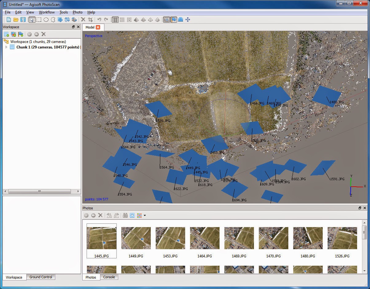
Figure 14: Next, a point cloud was generated for the images by selecting the Workflow tab and choosing the Align Photos option. Default values were accepted.

Figure 15: Next, a TIN was created from the point cloud by selecting the Workflow tab and choosing Build Mesh. Default values were accepted.

Figure 16: Finally, a texture was made by selecting the Workflow tab and choosing Build Texture and the view was changed to view the texture over the TIN. This is the resulting mosaicked image of the Bollinger Fields soccer fields.
The same process, starting at figure 12, was used to create a mosaicked orthoimage of the SX260 imagery.
Results

Figure 17: The resulting exported jpeg of the mosaicked ELPH imagery. For some reason the image came out rotated and skewed. The location information added to the images was accurate and the process was run multiple times, however the image always came out this way.

Figure 18: The resulting exported jpeg of the mosaicked SX260 imagery. This time the image came out in the proper orientation, however, it's a little dark.

Figure 19: The resulting mosaicked SX260 imagery with enhanced brightness and contrast.
Conclusions
The resulting mosaicked images look much better than what was expected. The idea that the string holding the balloon in place would be visible in the final image turned out to be false. PhotoScan did a great job at mosaicking the imagery together. Part of the reason the string did not show up in the final product was the extensive overlap of images. The enhanced image created from the SX260 imagery turned out the best as it covers the entirety of the soccer fields at Bollinger Fields and has a proper orientation.
Using only 20-30 images may have resulted in less accuracy in the final product. However, classmates that ran the mosaic with more images (200+) said the run time took hours to days to complete. Having the most accurate result was not the point of the activity however, and by using a smaller number of images, multiple mosaicked images of the study area were created in much less time.
The entire process of collecting imagery and creating a seamless mosaicked image was highly rewarding. Aside from filtering through the large number of mostly useless images, the hardest part of the process was actually collecting the imagery in the field. The mosaicking process was not incredible complicated, though to be fair most of the default values were kept when running the tools and the process could have been further refined adding complexity. This activity was a great introduction into the field of aerial imagery collection and processing, which I will be expanding upon in future classes.
Imagery Sources
UWEC Geospatial Field Methods Class Spring 2014
No comments:
Post a Comment