UWEC's spring 2014 semester now comes to a close and it's time to take a look back at the semester and recap all the methods and techniques I have learned by taking Geospatial Field Methods. In general, my technical geospatial knowledge has increased dramatically because not only was I taking this course, but GIS I and Remote Sensing as well. This class, however, has given me hands-on field experience that the other two did not, or only did slightly.
The semester started with Field Activity #1 and Field Activity # 2. In these activities, students built a miniature landscape in the snow, constructed a coordinate system for the landscape, and developed models to visualize the landscape. Students were expected to research and make these models themselves with little guidance. As a result, I was able to learn quite a bit about the different methods to create surfaces available in ArcMap and really just how to use ArcMap in a general sense.
Activity #3 was the most open ended activity of the semester and was meant to get students familiar with UAV technologies for later in the semester. Though this activity I learned the basics about UAS and the similarities and differences between rotocopters and fixed wing crafts. Having to research UAV's online was helpful later on during the equipment day and for completing Field Activity # 9.
The first survey of the semester was accomplished in Field Activity #4 when students preformed a distance azimuth survey in an area of their choosing. During this activity, the concepts of azimuth and magnetic declination were explored and the proper use of a laser rangefinder was learned.
Activity #5 taught students how to preform distance bearing navigation, essential for later on in the semester during Field Activity #10. Not only were the navigation techniques learned, but the maps used for Field Activity #10 were also created. More ArcMap knowledge was gained during this activity as multiple grids needed to be made for the different coordinate systems needed.
The basics of creating a geodatabase with proper domains was the focus of Activity #6. Here students needed to construct multiple domains to collect microclimate data later in the semester. The geodatabase created during this activity was used for Field Activity #7.
In Field Activity #7, students collected microclimate data around the UWEC campus area and each groups data was combined to create one microclimate map for the entire campus. Through this activity, I learned how to import, collect, and export data from a GPS unit.
The second survey of the semester was accomplished with the use of a Topcon Total Station and GMS-2 GPS unit in Field Activity #8. Elevation data was collected for the newly developed campus mall area on UWEC's lower campus and a DEM was created in ArcMap by drawing on knowledge from Field Activity # 2. This activity helped to cement the process of using a Total Station to conduct a survey into my brain as I had used one before.
Multiple class periods were spent at Bollinger Fields testing different UAV platforms which is detailed in Field Activity #9. After different imagery was collected, it was up to the students to figure out how to embed locational data into images and mosaic them together.
In Field Activity #10 and Field Activity #11 the navigation course at the Priory in the Town of Washington, WI was completed through different means. At first the course was partially completed though use of traditional means, a map and compass. Then the course of fully completed through use of a GPS unit. This let students compare the two approaches while also learning how to navigate rough terrain.
My favorite activities of the semester were the ones where the result felt the most rewarding. These activities were the ones were students needed to go out, collect data, and make models from the data. Collecting data for the microclimate maps was not enjoyable because of the bitter cold winds that day but the resulting maps of Field Activity #7 were worth it. Examining precipitation and wind patterns on campus was interesting and the wind direction map is definitely my favorite. Making the DEM through Field Activity #8 was greatly rewarding because the whole process was the most involved of the whole semester and the final result modeled the landscape very well. Remote sensing technologies and aerial imagery analysis has become my favorite topic as the semester has progressed and as a result, Field Activity #9 was the most enjoyable for me. Mosaicking the imagery collected as a class into one seamless image was surprisingly rewarding and really got me thinking about the applications of such techniques.
Overall, I feel I have learned an incredible amount this semester and the hands-on approach of this class helped a great deal. Taking this class is a requirement for obtaining the Geospatial Technique Certificate offered at UWEC but even if it wasn't, I would still recommend the class to any Geography major or anyone interested in a job which involves field work in the future.
Sunday, May 11, 2014
Field Activity #11: GPS Navigation
Introduction
For the final week of class, students went back to the Priory and completed the entire navigation course with the aid of a Trimble Juno 3B GPS unit. Any data or imagery loaded onto the GPS unit could be used. It was up to the individual groups to decide what to include and what would just be clutter. Each group will start at a different flag and complete the course in whichever manner they deem the best, taking a point with the GPS unit at every flag. Being the last class of the semester, paintball was incorporated into the activity for fun. There would be five teams of three students each competing to complete the course first. If someone was hit, their team would need to wait about 1 minute before moving on.
Methods
The process of creating a geodatabase and collecting data with ArcPad is explained in pervious blog posts Field Activity #7 and Lab 5 (from my GIS I blog).
Figure 1: Screenshot of what was exported to the GPS unit. The no shooting zone polygons indicate areas were children or other Nature Academy related personal may be present. The flag positions were kept small and the navigation path was kept skinny so they would be a appropriate size on the smaller Juno 3B screen. The 5 meter contour lines and study area was kept for reference. NavigationGroup3 is the point feature class that will be used during the activity to mark the location of the flags.
Group 3 began at flag number 10 and followed the purple line seen in Figure 1 until the final flag, number 1. The GPS unit was used as a interactive map for this navigation exercise. As the location of the GPS on the screen moved, we were able to have a better idea if we were close to the next flag or not. When a flag was reached, the GPS was held under it and a NavigationGroup3 point was taken in ArcPad. The process of watching the GPS unit and taking points at flags continued until point 6 was found. At that point it was almost after 6 and the activity ended.
Discussion
Figure 2: This is a map made for reference. It illustrates the starting and ending point and the general path taken to complete the course.
The navigation path taken was largely based on x,y location and less consideration was put into elevation. The difficulty due to elevation was visually approximated and ended up making the course pretty physically exhausting. The longest portion of the course was the beginning. The class was given paintball equipment near flag 1 and students were not allowed to be seen with paintball guns and masks in any of the no shooting zones. As a result, to get to our starting position at flag 10, we had to traverse multiple wooded thorny slopes taking us at least 15 minutes. Despite our slow start we picked up speed in the middle of the course getting into two skirmishes with other groups along the way.
Because of the guess-and-check nature of the navigation method used, we often found ourselves veering from our intended path. As a result, we ended up having to backtrack up and down steep slopes and walk in large arcs to avoid drastic changes in elevation. It was less work to set up the geodatabase and load it onto the GPS unit than it was to manually plot points and calculate bearings like we did in Field Activity # 10. However, when it came to actually doing the navigation, the compass and map were more helpful. Using only the GPS unit was time consuming due to all the backtracking and course adjustment that was necessary. While with the compass and map, we had a clear direction of where to go next.
Figure 3: A map showing the locations of flags as provided for the class in yellow and the GPS locations collected in the field by Group 3 in green. The points match up very well for flags 6, 8, 9, and 13, moderately well for flags 2, 3, 4, 5, 10, 11, and 12, and poorly for flags 7, 14, and 15.
Conclusions
This activity is a prime example of how "older" techniques can be more useful then newer technologic solutions. Using only the GPS unit made navigating the course more time consuming then needed and ended up being incredibly tiring. Taking the proper time to accurately calculate bearings for use with a map and compass made navigating a portion of the course relatively simple and quick. One way the GPS unit was better then the map and compass was that we could actually tell if we were close to a flag or not. Naturally, the conclusion here is that using a map, compass, and GPS unit together to preform the navigation course would be ideal.
Sources
UWEC Department of Geography and Anthropology
UWEC Geospatial Field Methods Class Spring 2014
Field Activity #10: Traditional Navigation
Introduction
This activity is the continuation of Activity #5, in which students learned the basics of distance bearing navigation and developed navigation maps of the Priory in Eau Claire, WI. These maps will now be used by students at the Priory as they complete a pre-established navigation course with only a map and orienteering compass.
Study Area
The study area chosen for the navigation exercises is the Priory in Eau Claire, WI. This land was acquired by UWEC in October of 2011 and has since been used by the university in a variety of ways including being the new location of UWEC's Children's Center, now referred to as the Nature Academy, and being the location of a living-learning community in collaboration with the Ho-Chunk Nation. The area consists of 112 acres of mostly forested land which is the real focus of this activity.
Figure 1: The priory is located about 3 miles south of the UWEC campus area.
Figure 2: This map illustrates the elevation characteristics of the Priory through use of a DEM and contour lines. Without this elevation data, the Priory grounds seem flat in aerial imagery and it could be assumed that traversing the area would be relatively easy. However, the closeness of the 5 meter contour lines indicate the areas true characteristics. The elevation of the Priory grounds ranges from 310, near the course staring points, to 250, with multiple steep slopes.
Methods
The navigation course entails 15 white and orange "flags" hung in trees throughout most of the Priory grounds. Each flag has a number and a unique punch-stamp attached to it. To confirm that the flag has been reached, the unique punch-stamp is used on a laminated piece of paper. For this activity, each group was assigned 5 flags to locate using only their self generated maps and an orienteering compass.
Figure 3: Group 3 was assigned to start at point 11 and end at point 15. This map shows each flag location, the no shooting zones (for use in the following GPS navigation exercise, indicating residential areas and the Nature Academy), and the path taken to reach each point from 11 to 15.
The maps used for this activity did not have the flag locations on them. When students arrived at the Priory, each group was given their flag numbers along with the corresponding coordinates. The students then had to manually plot these points on their maps and find the bearing to each point. This process is detailed in a previous blog post, Activity #5. Two different maps were made for this activity, one with UTM coordinates and another with latitude and longitude. Once the flag positions had be plotted and the bearings to each found, the groups then ventured into the woods returning after finding the five flags assigned.
Each groups consisted of three students, each playing a role in the navigation process. One student (the navigator) used the map and compass to point another student (the runner) at an object in the direction of the next flag. Once the runner had reached the object (usually a tree in this case) the last student walked to the runner taking a pace count as they went. Through combined effort, each group of three repeated this process until each flag was found.
Figure 4: Here is Eric, posing with a map, taking his turn as the navigator.
Figure 5: Here Morgan, taking her turn as the navigator, is pointing the runner (myself) to the location of a flag.
Figure6: Here I am, taking my turn as the runner, posing with the last flag we needed to find.
Discussion
When starting out, Group 3 decided to use the latitude/longitude map first and switch to the UTM map after a couple flags had been found to compare the maps and determine if one coordinate system is better for this scale navigation than the other. We got our answer immediately. It took us the longest to find the first point because tying to accurately plot the position of the flags using the latitude/longitude coordinates was quite difficult.
We ended up plotting flag 11 near flag 15 and somehow found flag 14 first. After about a half hour of climbing up and down steep slopes, we regrouped, ditched the latitude/longitude map, and used the UTM map. After switching the coordinate system the flags were much easier to find. This makes sense because latitude and longitude are geographic coordinates which are useful at small scales. However, the navigation activity at the Priory was conducted on a large scale and as such a projected coordinate system such as UTM is far more accurate and useful.
Conclusions
This activity was not as difficult as I had thought it would be as I had never used a map and compass for navigation purposes before. The varied elevation and, at times, thick vegetation were a major obstacle but once we started using UTM coordinates the whole process went rater quickly and smoothly. As long as proper time is taken to find the points and measure the bearings accurately, using a map and compass is a great way to navigate.
Sources
UWEC Department of Geography and Anthropology
Google Earth
© 2014
Sunday, May 4, 2014
Field Activity #9: Aerial Imagery Collection and Processing
Introduction
For this multi-week exercise, students will collect aerial imagery in the field and mosaic the images together. The study area, Bollinger Fields, was chosen because it offered the best terrain for testing different unmanned aerial systems. Over the past few weeks, students have been introduced to several methods of obtaining aerial imagery. A kite, balloon, rotocopter, and rockets have been used at Bollinger Fields for imagery collection with varying results. The imagery collected through these tests, as well as the platforms that collected the data, will now be analyzed and the best imagery will be mosaicked together through use of AgriSoft's PhotoScan.
Imagery and Platform Discussion
All imagery collected of Bollinger Fields was taken by two different sensors, a Cannon ELPH 110 HS and a Cannon SX260 HS. Regular cameras were used to simplify the whole process. Ideally, just the actual sensor inside the camera would be used for the rotocopter to decrease its payload. But for the kite and balloon, payload is less of an issue. The Cannon SX260 HS recorded GPS locations for each of the images it took, however, the Cannon ELPH 110 HS did not. If imagery taken with the Cannon ELPH 110 HS was going to be used for processing later on, it would need to either be georeferenced or have a tracklog with GPS locations embedded into the pictures. No still imagery was collected via the rockets. Instead, video was captured by small sensors taped to the rockets side.
Images of the kite, a rocket, and two different rotocopters can be seen in a pervious blog post, Equipment Day.
The Kite
The first platform used to collect imagery was a 9-foot kite. This exercise was more of a demonstration of how imagery collection could be done with a kite and what aerial imagery looks like before it is processed. The kite was raised to a certain height, the Cannon ELPH 110 HS attached to a metal and string stabilizing contraption was hooked onto the kites string, and the kite was raised up some more.

 The imagery collected by the kite does not cover an extensive area and the height of the sensor was not high enough to be of much use. This was simply an intro to unmanned aerial systems and aerial imagery and will not be used for further processing.
The Balloon
The next platform used to collect imagery was a 5-foot diameter balloon. After the balloon was filled and raised up a bit, the Cannon ELPH 110 HS and the Cannon SX260 HS where attached to the balloon string in the same fashion the Cannon ELPH 110 HS was attached to the kite earlier. Then the balloon was raised quite a bit higher to make sure the images taken would cover a large enough area and have plenty of overlap. Next, students took turns holding the balloon as the class walked throughout Bollinger Fields to cover the entire study area.


Imagery collected by the balloon was the best of all the platforms and therefore will be used for further processing. There is one problem with this imagery however, the balloon string can be seen in many of the pictures. As a result, finding pictures that were mostly vertical (non oblique) that did not also have a string plainly visible was difficult to do and there may be some string showing up in the final mosaicked image.
The Y6
The final platform used to collect imagery was our professor's rotocopter, the Y6. The Cannon SX260 HS was attached to the Y6 through use of metal screws and braces. The Y6 was being controlled through mission planning software via a laptop. Taking a zig-zaging pattern across the landscape, the Y6 collected imagery.


This imagery however turned out poorly as the contrast settings had been changed and little could be seen. On top of that, the time interval of photo capture, 2 seconds, was not enough to acquire imagery with enough overlap to properly mosaic. As a result, this imagery will not be used for further processing.
Methods
As stated above, the best imagery came from using the balloon and as such both sets of imagery captured that day will be used to create two separate mosaicked orthophotos of Bollinger Fields. Just over 300 images were collected for each camera and about 20-30 images each were selected to be mosaicked. The images selected were chosen because they were mostly vertical and collectively covered the entire study area. Only 20-30 images were chosen to reduce the processing time needed for PhotoScan to process the images.
Imagery captured with the SX260 was geotagged as the photographs were taken and as a result, the imagery was ready to be mosaicked. The imagery capture by the ELPH110 had no location data and information from a track log that has kept by the Y6 was needed in order for the imagery to be properly mosaicked.


The same process, starting at figure 12, was used to create a mosaicked orthoimage of the SX260 imagery.
Results


For this multi-week exercise, students will collect aerial imagery in the field and mosaic the images together. The study area, Bollinger Fields, was chosen because it offered the best terrain for testing different unmanned aerial systems. Over the past few weeks, students have been introduced to several methods of obtaining aerial imagery. A kite, balloon, rotocopter, and rockets have been used at Bollinger Fields for imagery collection with varying results. The imagery collected through these tests, as well as the platforms that collected the data, will now be analyzed and the best imagery will be mosaicked together through use of AgriSoft's PhotoScan.
Imagery and Platform Discussion
All imagery collected of Bollinger Fields was taken by two different sensors, a Cannon ELPH 110 HS and a Cannon SX260 HS. Regular cameras were used to simplify the whole process. Ideally, just the actual sensor inside the camera would be used for the rotocopter to decrease its payload. But for the kite and balloon, payload is less of an issue. The Cannon SX260 HS recorded GPS locations for each of the images it took, however, the Cannon ELPH 110 HS did not. If imagery taken with the Cannon ELPH 110 HS was going to be used for processing later on, it would need to either be georeferenced or have a tracklog with GPS locations embedded into the pictures. No still imagery was collected via the rockets. Instead, video was captured by small sensors taped to the rockets side.
Images of the kite, a rocket, and two different rotocopters can be seen in a pervious blog post, Equipment Day.
The Kite
The first platform used to collect imagery was a 9-foot kite. This exercise was more of a demonstration of how imagery collection could be done with a kite and what aerial imagery looks like before it is processed. The kite was raised to a certain height, the Cannon ELPH 110 HS attached to a metal and string stabilizing contraption was hooked onto the kites string, and the kite was raised up some more.
Figure 1: A class photo taken while the kite was being let up.
Figure 2: This was about the highest the kite went up. Because of the weather and all the snow on the ground it was decided that a walk through of Bollinger Fields to collect more imagery would wait for another day.
The Balloon
The next platform used to collect imagery was a 5-foot diameter balloon. After the balloon was filled and raised up a bit, the Cannon ELPH 110 HS and the Cannon SX260 HS where attached to the balloon string in the same fashion the Cannon ELPH 110 HS was attached to the kite earlier. Then the balloon was raised quite a bit higher to make sure the images taken would cover a large enough area and have plenty of overlap. Next, students took turns holding the balloon as the class walked throughout Bollinger Fields to cover the entire study area.
Figure 3: Here is a sample of the imagery taken with the ELPH 110. Notice the height difference compared to the imagery taken with the kite. Also take note of the string in the photo.
Figure 4: Here is a sample of imagery taken with the SX260. The contrast is markedly different then the imagery taken with the ELPH 110 even though the both where collected at the same time.
Imagery collected by the balloon was the best of all the platforms and therefore will be used for further processing. There is one problem with this imagery however, the balloon string can be seen in many of the pictures. As a result, finding pictures that were mostly vertical (non oblique) that did not also have a string plainly visible was difficult to do and there may be some string showing up in the final mosaicked image.
The Y6
The final platform used to collect imagery was our professor's rotocopter, the Y6. The Cannon SX260 HS was attached to the Y6 through use of metal screws and braces. The Y6 was being controlled through mission planning software via a laptop. Taking a zig-zaging pattern across the landscape, the Y6 collected imagery.
Figure 5: Samples of the imagery collected by the Y6 with the SX260. The day this platform was tested was quite windy and as a result it was kept a little to low to the ground. The resulting imagery did not cover an extensive area and the images did not overlay enough, if at all, for mosaicking.
This imagery however turned out poorly as the contrast settings had been changed and little could be seen. On top of that, the time interval of photo capture, 2 seconds, was not enough to acquire imagery with enough overlap to properly mosaic. As a result, this imagery will not be used for further processing.
Methods
As stated above, the best imagery came from using the balloon and as such both sets of imagery captured that day will be used to create two separate mosaicked orthophotos of Bollinger Fields. Just over 300 images were collected for each camera and about 20-30 images each were selected to be mosaicked. The images selected were chosen because they were mostly vertical and collectively covered the entire study area. Only 20-30 images were chosen to reduce the processing time needed for PhotoScan to process the images.
Imagery captured with the SX260 was geotagged as the photographs were taken and as a result, the imagery was ready to be mosaicked. The imagery capture by the ELPH110 had no location data and information from a track log that has kept by the Y6 was needed in order for the imagery to be properly mosaicked.
Figure 6: The file properties for an image taken by the ELPH 110. The GPS section in the Details tab is missing.
To add location data, a track log would need to be embedded into the imagery. This was accomplished through use of Geosetter.
Figure 7: The first screen that loads when Geosetter opens.
Figure 8: To load the desired ELPH 110 images, the folder with the green upwards pointing arrow was clicked in the upper left of the screen and the folder containing the photos was selected. Then the __ icon was clicked and the Synchronize with GPS Data Files window appeared.
Figure 9: The Synchronize with GPS Data Files window. Here the radio button for Synchronize with Data File was filled and the desired track log was chosen. All other default settings were kept and OK was clicked.
Figure 10: Now the images have location data associated with them as seen in the map section on the right. The images were then saved.
Figure 11: In the file properties for the new images, the GPS section has been generated.
Now that the selected imagery for the ELPH 110 had been given location data, the images could be opened in PhotoScan to be mosaicked. The selected imagery from the SX260 was already ready for the mosaicking process as stated above.
Figure 12: The first screen that loads when PhotoScan is opened.
Figure 13: To add the images, the Workflow tab was selected and Add Photos option was chosen. For this example, the ELPH imagery was selected.
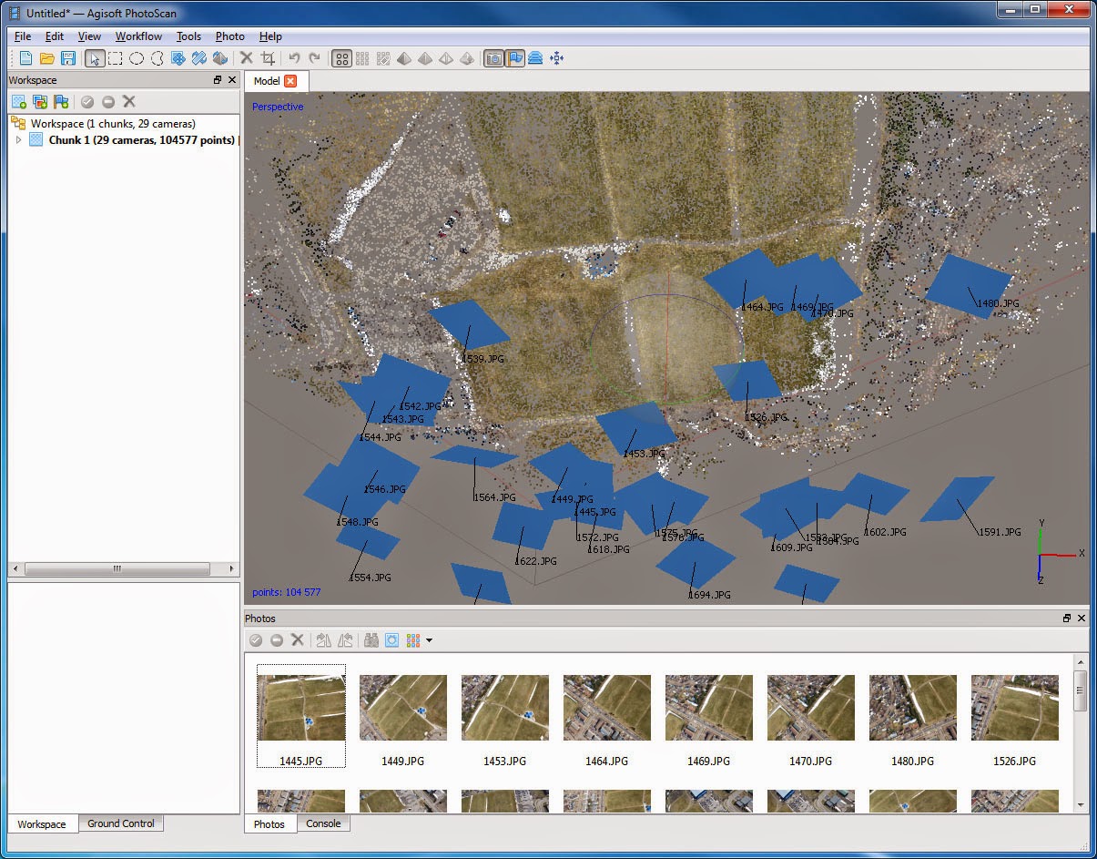
Figure 14: Next, a point cloud was generated for the images by selecting the Workflow tab and choosing the Align Photos option. Default values were accepted.
Figure 15: Next, a TIN was created from the point cloud by selecting the Workflow tab and choosing Build Mesh. Default values were accepted.
Figure 16: Finally, a texture was made by selecting the Workflow tab and choosing Build Texture and the view was changed to view the texture over the TIN. This is the resulting mosaicked image of the Bollinger Fields soccer fields.
The same process, starting at figure 12, was used to create a mosaicked orthoimage of the SX260 imagery.
Results
Figure 17: The resulting exported jpeg of the mosaicked ELPH imagery. For some reason the image came out rotated and skewed. The location information added to the images was accurate and the process was run multiple times, however the image always came out this way.
Figure 18: The resulting exported jpeg of the mosaicked SX260 imagery. This time the image came out in the proper orientation, however, it's a little dark.
Figure 19: The resulting mosaicked SX260 imagery with enhanced brightness and contrast.
Conclusions
The resulting mosaicked images look much better than what was expected. The idea that the string holding the balloon in place would be visible in the final image turned out to be false. PhotoScan did a great job at mosaicking the imagery together. Part of the reason the string did not show up in the final product was the extensive overlap of images. The enhanced image created from the SX260 imagery turned out the best as it covers the entirety of the soccer fields at Bollinger Fields and has a proper orientation.
Using only 20-30 images may have resulted in less accuracy in the final product. However, classmates that ran the mosaic with more images (200+) said the run time took hours to days to complete. Having the most accurate result was not the point of the activity however, and by using a smaller number of images, multiple mosaicked images of the study area were created in much less time.
The entire process of collecting imagery and creating a seamless mosaicked image was highly rewarding. Aside from filtering through the large number of mostly useless images, the hardest part of the process was actually collecting the imagery in the field. The mosaicking process was not incredible complicated, though to be fair most of the default values were kept when running the tools and the process could have been further refined adding complexity. This activity was a great introduction into the field of aerial imagery collection and processing, which I will be expanding upon in future classes.
Imagery Sources
UWEC Geospatial Field Methods Class Spring 2014
Subscribe to:
Comments (Atom)